---

What is a “Binary Classifier”?

Imagine you are working in the “Loan Department” of some bank. A farmer comes up with a loan application, and you are to approve or deny the loan. You will have to analyze several factors contributing to the risk of the loan being “defaulted”.

A loan is defaulted when the borrower is no longer deemed able to make the payments based on their agreement with the lender.

So, your job would be to answer the question - Should I approve this loan? Or in better terms - Will this loan be defaulted?

Note that, the final decision is binary (two outcomes): the loan is either Approved (Not Defaulted) or Denied (High Risk of Default). Your core challenge is predicting one of these two outcomes: Will the loan be classified as ‘Defaulted’ or ‘Not Defaulted’?”

While it may be fairly complicated for you to analyze all the data in the loan application and make the decision, a properly trained machine learning model can do this job for you in matter of seconds, if not milliseconds. That model would be a “binary classifier”.

Binary classifier is a machine learning model that tries to answer a yes/no question. Such question could be:

• Is this check fraudulent?
• Is this a spam email?
• Is this apple rotten?

A binary classifier attempts to “draw a boundary” separating the training dataset into two classes, for example Defaulted and Not Defaulted. When asked to make a prediction, it will essentially identify which “side” of the “decision boundary” the data point lies.

In this post, we will train such a binary classifier for the exact job discussed here - predicting whether a loan will default or not.

---

Setting up your environment

Here are a couple of things you should know before you start following along this post:

1. The code provided here is meant to be run in .NET Interactive environment like VS Code Polyglot Notebook.
2. The dataset used is downloaded from Kaggle. You can use some other dataset (even for training some other model altogether), but the code needs to be adjusted accordingly.

With that, here are the steps you should follow to set up the coding environment:

1. Create a new folder for the project.
2. Copy the downloaded dataset to the folder, and name it data.csv.
3. Open the folder in VS Code (or compatible code editor), and make sure the polyglot notebook extension is installed.
4. Create a new file with .dib extension. You can copy and paste the code in this post in the notebook and run it.

You should have replicated this folder structure:

LoanDefaultPrediction/
├── data.csv
└── LoanDefaultPrediction.dib

Also, before starting to work with the data and train the model, we should install a few NuGet packages. You can do this in the notebook with this code:

/**
Install NuGet packages:
1. Microsoft.Data.Analysis - Easy-to-use and high-performance libraries
for data analysis and transformation
2. Microsoft.ML - an open-source, cross-platform machine learning framework
for .NET developers that enables integration of custom machine learning
models into .NET applications
**/
#r "nuget:Microsoft.Data.Analysis"
#r "nuget:Microsoft.ML"

---

Playing with the data

First, we will inspect the data by loading the csv file in a DataFrame. For uniformity, we convert the column names to lowercase.

I highly recommend you to take a look at the columns description in Kaggle “Data Card” to get a better picture of the data we are working with.

using Microsoft.Data.Analysis;

const string DATASET_CSV_PATH = "./data.csv";

// Import the CSV file as DataFrame
DataFrame dataFrame = DataFrame.LoadCsv(DATASET_CSV_PATH);


foreach (var column in dataFrame.Columns)
{
    // Rename columns to lowercase
    dataFrame.Columns.RenameColumn(column.Name, column.Name.ToLower());
}

// Inspect the data
dataFrame.Head(5).Display();

As you may have noticed, the columns id and year do not help in making the prediction. So, we will remove these columns.

Also, the column that depicts whether the loan was defaulted or not is named status. For a binary classifier, this needs to be true or false instead of 0 and 1. So, we will convert this column to boolean.

The column we are predicting is called label while all other columns are called features in the context of binary classifier.

// Drop non-predictive columns - "id" & "year"
dataFrame.Columns.Remove("id");
dataFrame.Columns.Remove("year");

// The `label` we are interested in is the "status" column.
string labelColumnName = "status";

// Convert the numeric status column to boolean
// i.e, 1 to true and 0 to false
bool[] booleanStatuses = [..(dataFrame[labelColumnName] as SingleDataFrameColumn).Select(status => status == 1)];
dataFrame.Columns.Remove(labelColumnName);
dataFrame.Columns.Add(new PrimitiveDataFrameColumn<bool>(labelColumnName, booleanStatuses));


dataFrame.Head(5).Display();

---

Handling missing values

A machine learning model is a mathematical model, and has a hard time working with missing values. To overcome the challenge, we should replace the missing values with something else, for each column.

For categorical features, we will replace the null or empty values with unknown token. This has no significant impact on the training process, but improves the readability of the features.

For numeric features (like loan_amount and rate_of_interest), we will replace the null values with the mode of the feature.

Mode of a feature is the value with highest frequency. For example if the feature has values - 0, 1, 1, 2, 2, 2, 3, 4, 5, the mode is 2 because it occurs the highest number of times (3 times).

The code below iterates through each column, displays the top 10 most frequent values, and then fills missing values appropriately:

using System.IO;

// Store the distinct values for each features
Dictionary<string, string[]> distinctValues = [];

long numberOfRecords = dataFrame.Rows.Count;

// Display Top 10 Values (10 items with highest frequency) for each column
Console.Write("{0,-30}{1,-180}\n{2}", "Column", "Top 10 Values (By Frequency)", "".PadLeft(210, '-'));

const string missingValueReplacement = "unknown";

foreach (var column in dataFrame.Columns)
{
    bool isNumericColumn = column.IsNumericColumn();
    // Value Counts - a dataframe with all unique values with counts for each column
    // It has two columns - "Values" and "Counts"
    // Take only "Top 10 values"
    DataFrame valueCounts = column.ValueCounts().OrderByDescending("Counts");

    Console.Write($"\n{column.Name,-30}");

    // Display the Top 10 values
    List<string> values = [];
    for (int i = 0; i < Math.Min(10, valueCounts.Rows.Count); i++)
    {
        var value = valueCounts["Values"][i];
        string valueStr = isNumericColumn ? value.ToString() : string.IsNullOrEmpty(value.ToString()) ? missingValueReplacement : value.ToString();

        Console.Write($"{valueStr,-18}");

        if (!isNumericColumn)
        {
            values.Add(valueStr);
        }
    }

    // The "values" is populated only for categorical columns
    distinctValues.Add(column.Name, [..values]);

    // Fill the missing values in numeric columns with their MODE (item with highest freqeuncy)
    if (isNumericColumn)
    {
        var mode = (float) valueCounts["Values"][0];
        column.FillNulls(mode, inPlace: true);
        continue;
    }

    // Replace empty strings with missingValueReplacement for categorical columns
    for (int i = 0; i < numberOfRecords; i++)
    {
        if (string.IsNullOrEmpty(dataFrame[column.Name][i]?.ToString()))
        {
            dataFrame[column.Name][i] = missingValueReplacement;
        }
    }

}

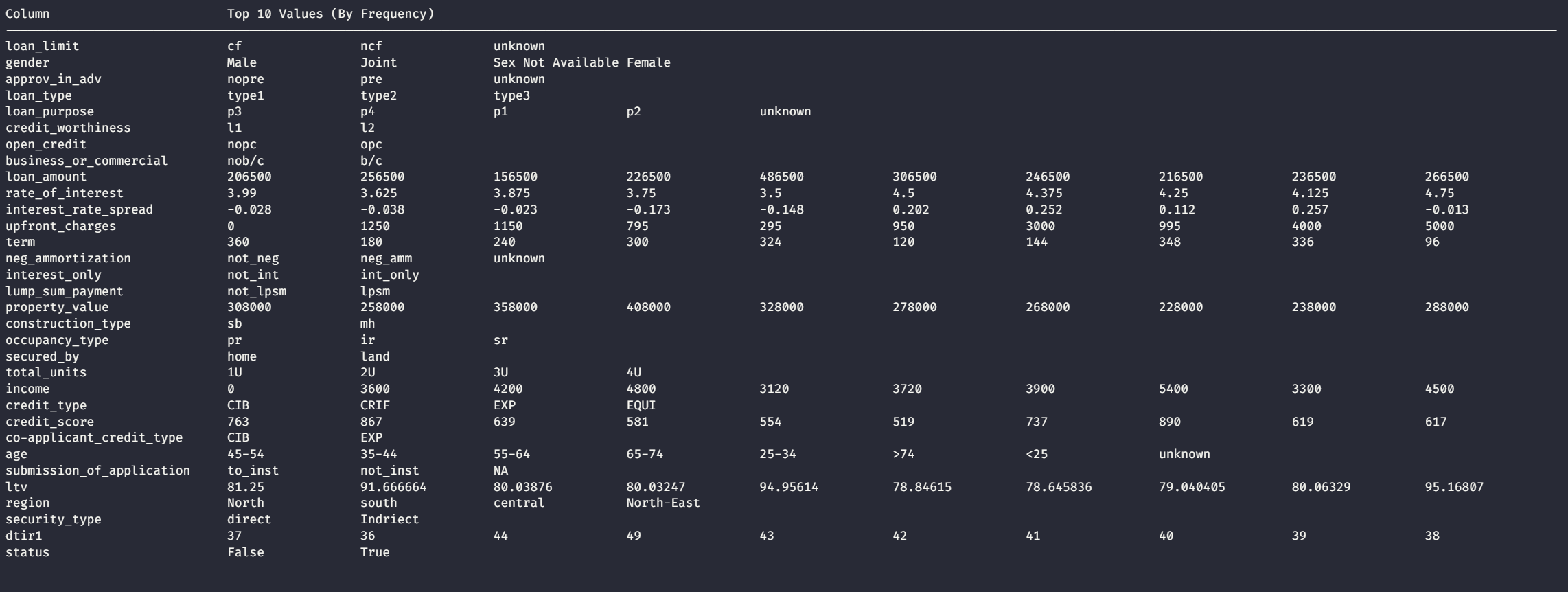
Top 10 values for each column, ordered by frequency. The first value for each column is its mode.

What’s happening here:

• The code displays the top 10 most frequent values for each column so you can see the data distribution
• For numeric columns, it fills missing values with the mode (most frequent value), which is a reasonable default
• For categorical columns, it replaces missing values with the string "unknown", making them explicit rather than leaving them as nulls
• The distinct values are stored for later use in the feature encoding table

The maximum number of unique (distinct) values for the categorical columns is 8 (for age). So, top 10 values is enough to capture ALL values for the categories.

---

Train-test split

If we use all available data to train the model, there is no way of evaluating it later. This would be like asking a student to cram answers of all possible questions of an exam, and then asking the student to take the same exam. So, we split the available data into two distinct sets. By distinct, we mean that they do not share any common records. These sets are called “training set” and “testing set”, and the process is called “train-test split”.

We will use the MLContext from Microsoft.ML (ML.NET) package to do this. If you haven’t noticed, we are now moving from “Data Analysis” to “Machine Learning” 🚀!

The ratio of data reserved for testing is called “split ratio”. We are using 15% as the split ratio. Generally, 10 to 30% of the data is reserved for testing.

using Microsoft.ML;

// Prepare the ML Context for feature selection, transformation and training
MLContext mlContext = new();

// Train test split
var trainTestData = mlContext.Data.TrainTestSplit(
    dataFrame,
    testFraction: 0.15 // 15% of the total data is used for testing and 85% for training
);

DataFrame trainData = trainTestData.TrainSet.ToDataFrame(maxRows: dataFrame.Rows.Count);
DataFrame testData = trainTestData.TestSet.ToDataFrame(maxRows: dataFrame.Rows.Count);

// Check to see if both status (true and false) are included in both data set
Console.WriteLine($"Training Dataset ({trainData.Rows.Count}/{dataFrame.Rows.Count})");
trainData.Head(5).Display();

Console.WriteLine($"Testing Dataset ({testData.Rows.Count}/{dataFrame.Rows.Count})");
testData.Head(5).Display();

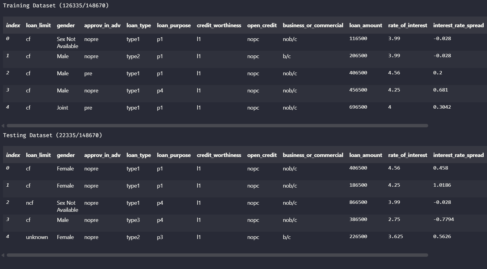
A preview of training and testing dataset produced after splitting.

It is important to make sure that both classes - status = True and status = False are included in both training and testing data set. There are methods to do so (see this GitHub issue about stratified splitting), but we will rely on the default split for now. In any case, you should verify this by inspecting the dataframes.

---

Preparing the data for training

This is probably the most crucial part of the whole training process. We will create a data processing pipeline that does the following:

1. One-Hot encode the categorical features

One-Hot encoding is one of the encoding techniques for converting categorical features to numeric. We essentially create one new binary feature (possible values are 0 or 1) per distinct value of the category. Then, we assign 1 for the “hot” feature and 0 for the “cold” ones.

For example, consider the gender feature. The distinct values are:

• Female
• Joint
• Male
• Sex Not Available

So, the gender feature is converted to 4 numeric features: gender_Female, gender_Joint, gender_Male, and gender_Sex_Not_Available. For a record with gender = Female, these numeric features will have values 1, 0, 0, 0 respectively. Since only “one” numeric feature is “hot” per category, the name is “one-hot” encoding. This transformation is necessary because machine learning algorithms work with numbers, not text.

2. Features concatenation

After all the features are numeric, we combine them into a single vector. The only relevant columns for training are features (all input variables) and status (our label/target to predict). This is equivalent to the X matrix and y vector in traditional statistics or regression problems.

3. Normalize the features

Finally, we normalize the features column so that it has zero mean and unit variance. Normalization ensures that all features are on the same scale—preventing features with large values from dominating the training process. This significantly improves the stability and speed of the training algorithm.

using Microsoft.ML.Data;

// Name of features column
const string featuresColumnName = "features";
const string normalizedFeaturesColumnName = "normalized_" + featuresColumnName;

DataFrameColumn[] featureColumns = [..trainData.Columns
    .Where(column => column.Name != labelColumnName)];

IEstimator<ITransformer> dataProcessingPipeline =
// encode categorical features - convert string values to numeric
mlContext.Transforms.Categorical.OneHotEncoding([
    ..featureColumns.Where(column => !column.IsNumericColumn())
        .Select(column => new InputOutputColumnPair(column.Name))
],
keyOrdinality: Microsoft.ML.Transforms.ValueToKeyMappingEstimator.KeyOrdinality.ByValue)
// features concatenation - combine all relevant features to a single vector
.Append(mlContext.Transforms.Concatenate(featuresColumnName, [
    ..featureColumns.Select(column => column.Name)
]))
// normalize features - transform for mean = 0 and variance = 1
.Append(mlContext.Transforms.NormalizeMeanVariance(
    outputColumnName: normalizedFeaturesColumnName,
    inputColumnName: featuresColumnName
));

// Inspect the transformed data
// The features vector has 1 element per numeric feature
// and N elements per cateogircal feature with N distinct values.
var previewData = dataProcessingPipeline
    .Fit(trainData)
    .Transform(trainData)
    .Preview(maxRows: 5);

// See the "Hot Features"
// All numeric 'features' are "hot" because every row has the value for them
// Categorical features are "hot" only if the row has the value equal to the category it represents
Console.WriteLine("{0,-90}{1,10}\n{2}", "hot " + featuresColumnName, labelColumnName, "".PadLeft(100, '-'));

foreach (var row in previewData.RowView)
{
    VBuffer<Single> features = (VBuffer<Single>) row.Values.FirstOrDefault(rowValue => rowValue.Key == featuresColumnName).Value;

    var label = row.Values.FirstOrDefault(rowValue => rowValue.Key == labelColumnName).Value;
    var allFeatures = features.Items().ToArray();
    var hotFeatures = allFeatures.Select(item => item.Key);

    Console.WriteLine("{0,-90}{1,10}", string.Join(" ", hotFeatures), label);
}

Hot features preview showing the “hot” features among 74 total features

The code block above demonstrates the data processing pipeline and displays a preview of the transformed data. You’ll notice that only the feature indices with “hot” values are shown—these correspond to the features present in each record. This sparse representation saves memory since categorical features with many distinct values can create many zero columns.

Note that the features column uses sparse vectors—storing only non-zero elements as key-value pairs to preserve memory. Each pair contains the feature index and its value, avoiding the need to store all the zeros.

To make sense of the numeric indices in the features vector, the following code block generates a mapping table. This is especially useful after one-hot encoding, where a single categorical column becomes multiple numeric columns. Understanding this mapping will also help you interpret feature contributions in the model’s predictions.

// See the feature behind each index in the feature column
// produced after "One-Hot Encoding" the categories
// and concatenating them with numeric features

// The display result is also useful to understand feature contributions
// in the predictions, made at the end in the notebook.

Console.WriteLine($"{"Index", -20}{"Feature", -30}{"Value", -30}\n{"".PadLeft(70,'-')}");

int index = 0;
foreach (var column in featureColumns)
{
    string[] values = column.IsNumericColumn() ? [""] : [..distinctValues[column.Name].Order()];

    foreach (var value in values)
    {
        Console.WriteLine($"{index, -20}{column.Name, -30}{value, -30}");
        index++;
    }
}

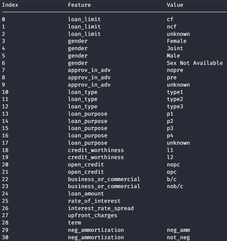
A table showing the feature (and value for categories) for each index in the feature array. This table is refered as “one-hot” encoding table.

---

Training and evaluating the model

Finally, we are ready to train the classifier model 🙌. We will be using LbfgsLogisiticRegression trainer - which is just one of many algorithms we can use to train the binary classification model.

In addition to making the prediction, we can also see which features influenced the decision the most. For that purpose, we have added feature contribution pipeline in the model.

After training the model, we are also evaluating the model against the testing data set. This evaluation gives some useful metrics about the model.

A prediction of status = True is “positive”. If it is correct, it is a true positive. Otherwise, it is a false positive. Similarly, a prediction of status = False is “negative”. If it is correct, it is a true negative. Otherwise, it is a false negative.

Some easy to understand metrics that help us see how good is the model are:

1. Precision: It is the ratio of true positives to total positives.
2. Accuracy: It is the ratio of correct predictions (true positive + true negative) to total number of predictions.
3. Recall: It is the ratio of correct positive predictions to actual positive values.
4. F1 Score: It is harmonic mean of precision and recall.
5. Confusion Matrix: It represents four main metrics - true positive, false positive, true negative and false negative.

Ideally, we should have precision, accurary, recall and F1 score close to 1. Similarly, the false positive and false negative count shooud be close to 0.

// Train the model
var trainer = mlContext.BinaryClassification.Trainers.LbfgsLogisticRegression(
    labelColumnName: labelColumnName,
    featureColumnName: normalizedFeaturesColumnName
);

var model = dataProcessingPipeline.Append(trainer).Fit(trainData);

// to enable feature contributions
var modelWithFc = model.Append(mlContext.Transforms
    .CalculateFeatureContribution(model.LastTransformer)
    .Fit(dataProcessingPipeline.Fit(trainData).Transform(trainData)));

// Evaluate the model
var predictions = modelWithFc.Transform(testData);

var metrics = mlContext.BinaryClassification.Evaluate(
    data: predictions,
    labelColumnName: labelColumnName,
    scoreColumnName: "Score"
);

metrics.Display();

// Save the model for future use
mlContext.Model.Save(modelWithFc, (dataFrame as IDataView).Schema, "./model.zip");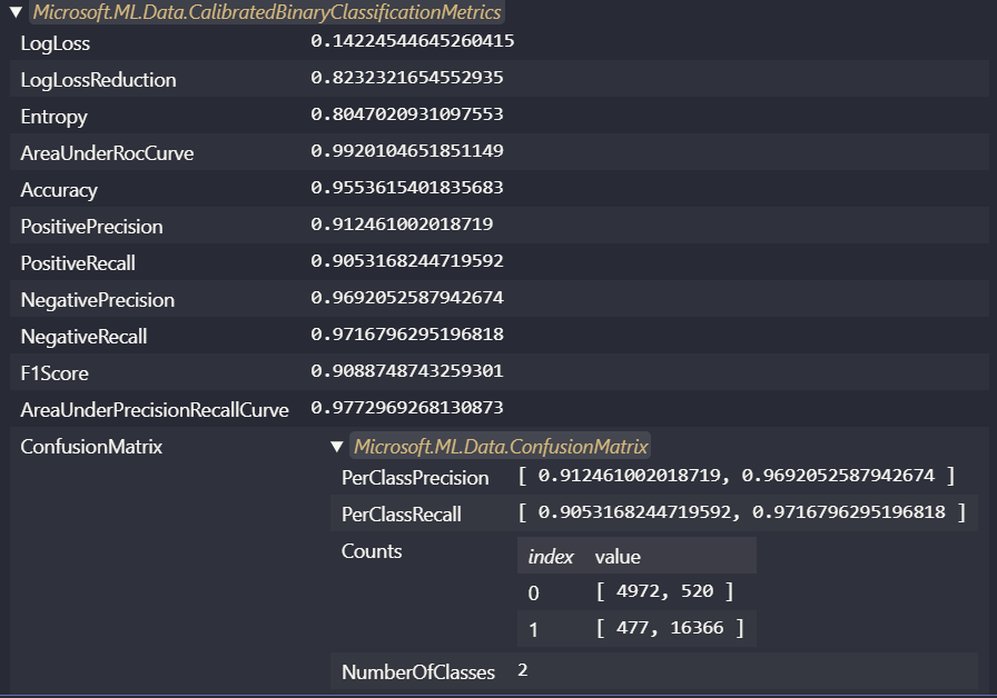

Metrics for a sample training.

---

Making predictions

After saving the model as a zip file, we can use it later for making one-time predictions (or in batch - but that is not covered in this post). But, first we need to define the “observation” and “prediction” classes.

The observation class has properties corresponding to the column names (and indices) we had in the training dataset. This is necessary so that the model can run the data processing pipeline and produce the features matrix properly.

The default values in the observation class are the modes we computed while displaying the “Top 10 Values”.

The prediction class has some properties that are useful in interpreting the prediction:

• PredictionLabel: This is the predicted status of the loan. It can be True or False.
• Probability: This is the probability (or confidence) of the loan being defaulted. It is high for PredictedLabel = True and low otherwise.
• FeatureContributions: This contains the weight of each feature in the prediction. More relevant features correspond to higher values. To interpret the features contribution, we should use the “One-Hot” encoding table.

// Defining classes for predictions
public class LoanDefaultObservation
{
    [LoadColumn(0), ColumnName("loan_limit")]
    public string LoanLimit = "cf";

    [LoadColumn(1), ColumnName("gender")]
    public string Gender = "Male";

    [LoadColumn(2), ColumnName("approv_in_adv")]
    public string ApprovedInAdvance = "nopre";

    [LoadColumn(3), ColumnName("loan_type")]
    public string LoanType = "type1";

    [LoadColumn(4), ColumnName("loan_purpose")]
    public string LoanPurpose = "p3";

    // Columns 5 to 26 omitted for brevity
    // The complete code is in the GitHub Gist notebook

    [LoadColumn(27), ColumnName("ltv")]
    public float LoanToValue = 81.25f;

    [LoadColumn(28), ColumnName("region")]
    public string Region = "North";

    [LoadColumn(29), ColumnName("security_type")]
    public string SecurityType = "direct";

    [LoadColumn(30), ColumnName("dtir1")]
    public float DebtToIncome = 37;
}

public class LoanDefaultPrediction
{
    public bool PredictedLabel;
    public float Probability;
    public float[] FeatureContributions;

    public override string ToString()
    {
        return @$"Probability of Defaulting:      {this.Probability}
Defaulted:                      {this.PredictedLabel}
Highest Contributing Features:  {string.Join(", ", this.FeatureContributions
    .Select((contrib, index) => (index, contrib))
    .Where(fc => fc.contrib != 0)
    .OrderByDescending(fc => fc.contrib)
    .Take(5))}
";
    }
}

And finally, the code to make the predictions is given below. Notice how we are creading a new context and loading the saved model instead of reusing the one used for training (and testing). Although the model is exactly the same, you would train once and reuse the saved model time and again.

// Making a prediction using the saved model
var predictionContext = new MLContext();

var predictionModel = predictionContext.Model.Load("./model.zip", out var modelSchema);

var predictionEngine = predictionContext.Model
    .CreatePredictionEngine<LoanDefaultObservation, LoanDefaultPrediction>(predictionModel);

LoanDefaultObservation[] sampleObservations = [

// This sample is very close to a sample that defaulted.
// So, expect the prediction to "Defaulted = True"
new()
{
    Gender = "Female",
    LoanPurpose = "p1",
    LoanAmount = 118500,
    PropertyValue = 120000,
    Income = 2000,
    CreditType = "EXP",
    CreditScore = 750,
    Age = "25-34",
    LoanToValue = 100f,
    Region = "south",
    DebtToIncome = 45
},

// This sample is very close to a sample that didn't default.
// So, expect the prediction to "Defaulted = False"
new(){
    ApprovedInAdvance = "pre",
    LoanPurpose = "p1",
    LoanAmount = 400000,
    RateOfInterest = 4.5f,
    InterestRateSpread = 0.2f,
    UpfrontCharges = 600,
    PropertyValue = 500000,
    Income = 10000,
    CreditType = "EXP",
    CreditScore = 850,
    Age = "35-44",
    LoanToValue = 80f,
    Region = "south",
    DebtToIncome = 45,
}];

LoanDefaultPrediction[] predictions = [..sampleObservations.Select(sample => predictionEngine.Predict(sample))];

// See the predictions
// To understand which features are contributing most,
// tally the feature index with the one-hot encoding table

Console.WriteLine(string.Join("\n\n", predictions.Select((prediction, index) => $"LOAN OBSERVATION {index + 1}\n{"".PadLeft(20, '-')}\n{prediction}")));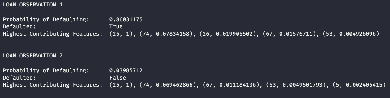

Predictions made for two sample observations.

---

Final notes

Congratulations! You’ve successfully built, trained, and evaluated a binary classifier for loan default prediction. But this is just the beginning.

Next steps you might consider:

1. Hyperparameter tuning: The LbfgsLogisticRegression trainer has parameters like learning rate and regularization strength that you can adjust to potentially improve model performance. Experiment with different values and measure the impact on your test metrics.

2. Try other algorithms: Logistic regression is just one approach. ML.NET also supports decision trees, gradient boosting, and neural networks. Different algorithms may perform better on this specific dataset.

3. Cross-validation: Instead of a single train-test split, use k-fold cross-validation to get a more reliable estimate of model performance across different subsets of data.

Common pitfalls to avoid:

• Data leakage: Never use information from the test set during training or preprocessing. We avoided this by splitting the data first.
• Overfitting: A model that memorizes training data performs poorly on new, unseen data. Monitor your test metrics closely.
• Ignoring the business context: In lending, false negatives (approving loans that default) and false positives (rejecting loans that wouldn’t default) have different costs. A precision of 95% might be insufficient if most of your false positives are rejections of good applicants.

Deploying your model:

Once you’re satisfied with performance, you can save the model (as we did with model.zip) and integrate it into a production system. ML.NET supports deployment to web services, Azure, or directly into .NET applications.

For deeper learning, explore the resources in the References section, and experiment with different datasets and approaches. The best way to master machine learning is through hands-on practice. Happy coding!

References

• ML.NET
• Loan Default Dataset
• GitHub Gist with Source Code

---

Next in the Series - Synthetic Data Generation using Cumulative Distribution Functions

---

You can read this post in Medium.

---