Synthetic Data Generation using Cumulative Distribution Functions
Have you ever wondered how synthetic data is generated to extend empirically collected sample data? I discuss one statistically justifiable approach to solve this problem in this post - by using cumulative distribution functions (CDFs).
Previous in the Series - Loan Default Prediction with Binary Classifier
Why synthetic data?
Traditionally, supervised machine learning models are developed using labeled datasets, where the target variable (the outcome) is known. This allows the model to learn relationships and be validated against a “ground truth.” In a production environment, however, the model encounters inference data, where the outcome is unknown at the time of prediction.
While recorded data is the gold standard, synthetic data generation is essential for simulating complex real-world scenarios. It allows developers to stress-test models against edge cases, ensure privacy compliance by removing PII, and validate system architecture before sensitive real-world data is available.
The use case I am going for is a little unconventional. I am making a web based game, and want to use the synthetic data for an engaging gameplay.
Getting started
I am going to refer to code snippets from the interactive notebook, which assumes a couple of things:
- You have trained a binary classifier model using the
train-model.csscript. The process is almost identical to the one explained in the loan default prediction blog post. - You have prepared both the trained model (
model.zip) and the processed data (processed-data.csv).
Also, before starting to work with the data and train the model, we should install a few NuGet packages:
- Microsoft.Data.Analysis - To load the processed data as data frame and work with it.
- Microsoft.ML - To load pre-trained model and make predictions
- Plotly.NET - To visualize data distribution and visually verify the closeness of synthetic data.
You can use this snippet to install the required packaged through the interactive notebook:
#r "nuget: Microsoft.Data.Analysis, 0.23.0"
#r "nuget: Microsoft.ML, 5.0.0"
#r "nuget: Plotly.NET, 6.0.0-preview.1"
#r "nuget: Plotly.NET.CSharp, 0.14.0-preview.1"
#r "nuget: Plotly.NET.Interactive, 6.0.0-preview.1"
Preparing the dataset
Before generating synthetic data, we need to prepare the dataset by loading it and computing the baseline loan default rate. This metric serves as a reference point that we’ll compare against the synthetic data we generate later to ensure our generation process produces realistic distributions.
We also remove the status column (our target variable) and the ltv column (which we’ll derive later from other features) from the data preparation.
using Microsoft.Data.Analysis;

DataFrame dataFrame = DataFrame.LoadCsv("./processed-data.csv");


int totalDefaulted = dataFrame["status"].Cast<bool>()
    .Where(status => status).Count();

Console.WriteLine($@"
Loan Default Rate: {Math.Round(100f * totalDefaulted/dataFrame.Rows.Count, 2)}%
");

// we don't want to generate data for status and ltv (loan_amount / property_value)
string[] skippedColumns = ["status", "ltv"];

foreach( var columnName in skippedColumns)
{
    dataFrame.Columns.Remove(columnName);
}

dataFrame.Head(5).Display();
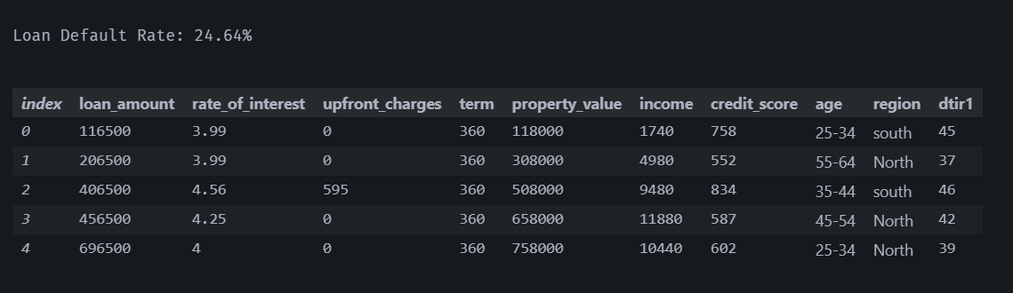
Next, we examine the distinct values in categorical columns. The age and region columns contain categorical values (like “<25”, “North-East”) which need to be converted to numeric values to derive cumulative distribution functions. By examining all distinct values first, we can create appropriate mappings for the conversion.
// see the distinct values for age and region
dataFrame["age"].Cast<string>().Distinct().Display();
dataFrame["region"].Cast<string>().Distinct().Display();
age and region columnsTo derive cumulative distribution functions, we need all columns in numeric form so they can be sorted. For the age column, we map each age group to its midpoint (for example - “25-34” to 30), which reasonably represents the age group. For the region column, we use an arbitrary numeric mapping (for example - “North-East” to 1) since regions have no inherent ordering. Once converted, the DataFrame is fully numeric and ready for CDF computation.
// for age we map to their group averages
var floatAges = dataFrame["age"].Cast<string>()
    .Select(age => age switch
    {
        "<25" => 20f,
        "25-34" => 30f,
        "35-44" => 40f,
        "45-54" => 50f,
        "55-64" => 60f,
        "65-74" => 70f,
        ">74" => 80f,
        _ => 0f
    });

dataFrame["age"] = new SingleDataFrameColumn("", floatAges);

// for region we use arbitrary mapping
var floatRegions = dataFrame["region"].Cast<string>()
    .Select(region => region switch
    {
        "North-East" => 1f,
        "North" => 2f,
        "central" => 3f,
        "south" => 4f,
        _ => 0f
    });

dataFrame["region"] = new SingleDataFrameColumn("", floatRegions);

dataFrame.Head(5).Display();

Histograms
A histogram is a graphical representation of the distribution of a dataset, showing the frequency of values within specified ranges (bins). By visualizing histograms for each column, we can see the shape and spread of the data—whether it’s normally distributed, skewed, or multimodal. Later, we’ll generate synthetic data and compare these histograms side-by-side to verify that our synthetic data preserves the empirical distributions found in the original dataset. This visual verification is crucial for ensuring the synthetic data’s statistical validity.
using Plotly.NET.CSharp;

foreach (var column in dataFrame.Columns)
{
    Chart.Histogram<float, string, string>(
        X: new(column.Cast<float>(), true),
        HistNorm: Plotly.NET.StyleParam.HistNorm.Percent
    )
    .WithXAxisStyle<float, string, string>(column.Name)
    .Display();
}
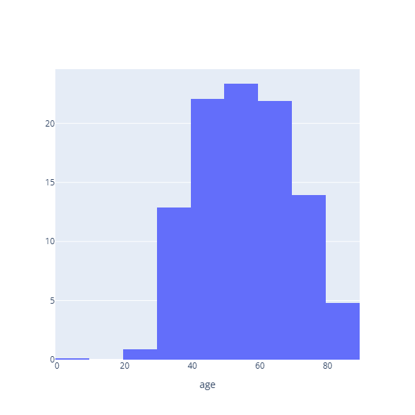
age column for the empirical data.Cumulative Distribution Functions (CDFs)
A Cumulative Distribution Function (CDF) represents the probability that a random variable is less than or equal to a specific value.
Let’s consider the following freqeuncy table. The cumulative frequencies and probabilities are derived from the frequencies of respective values.
| SN | x | f | Cumulative Frequency (cf) | Probability: P(X<=x) |
|---|---|---|---|---|
| 0 | 1 | 3 | 3 | 3/16 |
| 1 | 2 | 5 | 3 + 5 = 8 | 1/2 |
| 2 | 3 | 2 | 8 + 2 = 10 | 5/8 |
| 3 | 4 | 2 | 10 + 2 = 12 | 3/4 |
| 4 | 5 | 4 | 12 + 4 = 16 | 1 |
The CDF (the mapping from X to probability) tells us that there’s a 75% probability of the value being less than or equal to 4.
To generate synthetic data, we generate random probabilities (between 0 and 1) and find the corresponding values from the CDF through inverse transformation. This ensures our synthetic data follows the same probability distribution as the original data.
We are limiting samples up to 20 unique values per column to create compact yet representative CDFs that are efficient to store and use.
using System.IO;
using System.Text.Json;

// "column_name" : {<x> : <probabilities>}
Dictionary<string, Dictionary<float, float>> cdfs = [];

foreach (var column in dataFrame.Columns)
{
    DataFrame valueCounts = column.ValueCounts().OrderBy("Values");

    long[] counts = [..valueCounts["Counts"].Cast<long>()];
    long totalCount = counts.Sum();

    float[] probabilities = [
        ..Enumerable.Range(0, counts.Length)
        .Select(index => 1f * counts[0..(index + 1)].Sum() / totalCount)
    ];

    valueCounts.Columns.Add(new PrimitiveDataFrameColumn<float>(
        name: "Probabilities",
        probabilities
    ));

    // only keep 20 unique values per column
    int maxRows = 20;
    long numberOfRows = valueCounts.Rows.Count; // count of unique values

    if (numberOfRows > maxRows)
    {
        var step = Math.Ceiling(1f * numberOfRows / maxRows);
        var numberOfIndices = (int) Math.Ceiling(1f * numberOfRows / step);

        long[] indices = [
            ..Enumerable.Range(0, numberOfIndices)
                .Select(index =>  index * (int) step)
        ];

        // make sure that the last index is included
        indices[^1] = numberOfRows - 1;

        valueCounts = valueCounts.Filter(new PrimitiveDataFrameColumn<long>(
            "", indices
        ));
    }

    float[] cdfValues = [..valueCounts["Values"].Cast<float>()];
    float[] cdfProbabilities = [..valueCounts["Probabilities"].Cast<float>()];

    // empirical CDF for the column
    Dictionary<float, float> cdf = cdfValues
        .Zip(cdfProbabilities, (value, probability) => new {value, probability})
        .ToDictionary(kv => kv.value, kv => kv.probability);

    cdfs.Add(column.Name, cdf);

    // visualize CDF
    Chart.Line<float, float, string>(x: cdfValues, y: cdfProbabilities)
        .WithXAxisStyle<float, float, string>(column.Name)
        .WithYAxisStyle<float, float, string>("Cumulative Probability")
        .Display();
}

File.WriteAllText("./cdfs.json", JsonSerializer.Serialize(cdfs));
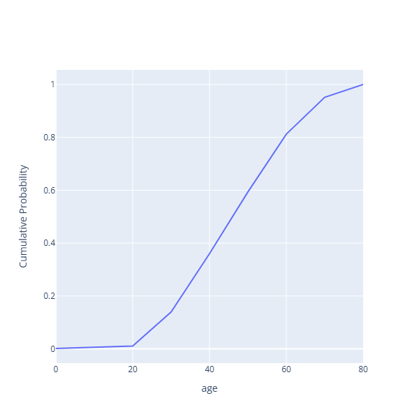
age columnBy serializing and saving the CDF tables to a JSON file, we create a reusable artifact that encodes the empirical probability distributions of the original data. This means we can generate as much synthetic data as needed without recomputing the CDFs each time. We can simply load the pre-computed CDFs and apply the inverse transformation.
This approach is efficient, reproducible, and can be easily shared or integrated into different parts of your application.
Generating synthetic data
The inverse CDF method is a powerful statistical technique for generating synthetic data. By generating a random probability (a uniformly distributed value between 0 and 1) and finding the corresponding value from the CDF, we create synthetic data points that follow the same probability distribution as the original data.
This works because of a fundamental probability theorem:
If U is uniformly distributed on [0,1] and we apply the inverse CDF to U, the resulting values follow the target distribution.
The code given below iterates through each column’s CDF, generates random probabilities, and selects the first CDF value whose cumulative probability exceeds the random value. This creates a new DataFrame where each column’s distribution matches the empirical distribution from the original data.
var random = new Random();

cdfs = JsonSerializer.Deserialize<Dictionary<string, Dictionary<float, float>>>(
    File.ReadAllText("./cdfs.json")
);

int numObservations = 1000;

// assumption: all the columns represent independent random variables
var syntheticData = new DataFrame(cdfs.Select(kv => new SingleDataFrameColumn(
    // kv.Key -> column_name
    // kv.Value -> <x> : <probability>
    kv.Key, Enumerable.Range(0, numObservations).Select(_ => {
        // generate CDF value (random value between 0 & 1)
        var probability = random.NextDouble();
        // find the "x" value that corresponds to the CDF value
        return kv.Value.First(kv => kv.Value > probability).Key;
    })
)));
To verify that our synthetic data authentically preserves the original distributions, we compare histograms of the synthetic data with those of the original data. By visualizing both datasets’ histograms side-by-side, we can visually inspect that they have similar shapes, spreads, and modes.
If the distributions match closely, it confirms that our inverse CDF generation process successfully captured the empirical characteristics of the original data, validating our approach.
// visually verify distribution
foreach (var column in syntheticData.Columns)
{
    Chart.Histogram<float, string, string>(
        X: new(column.Cast<float>(), true),
        HistNorm: Plotly.NET.StyleParam.HistNorm.Percent
    )
    .WithXAxisStyle<float, string, string>(column.Name)
    .Display();
}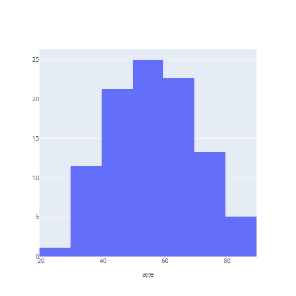
Histogram for the synthetic age column. Notice the resemblance with the
same for empirical age column.
Before we can make predictions on the synthetic data, we need to reverse our earlier transformations. The age and region columns must be converted back to their original categorical forms since the trained model expects these categorical features as inputs.
Additionally, we derive the ltv (loan-to-value) column by dividing loan_amount by property_value, completing the feature set required for the classifier.
// revert age and region columns
var stringAges = syntheticData["age"].Cast<float>()
    .Select(age => age switch
    {
        0 => "unknown",
        < 25 => "<25",
        < 35 => "25-34",
        < 45 => "35-44",
        < 55 => "45-54",
        < 65 => "55-64",
        < 75 => "65-74",
        < 85 => ">74",
        _ => "unknown"
    });

syntheticData["age"] = new StringDataFrameColumn("", stringAges);

var stringRegions = syntheticData["region"].Cast<float>()
    .Select(region => region switch
    {
        1f => "North-East",
        2f => "North",
        3f => "central",
        4f => "south",
        _ => "unknown"
    });

syntheticData["region"] = new StringDataFrameColumn("", stringRegions);

// compute ltv
syntheticData["ltv"] = syntheticData["loan_amount"] / syntheticData["property_value"];

syntheticData.Head(5).Display();
Completing the data with predictions
With the synthetic data prepared, we load our pre-trained binary classifier model and use it to predict the status (loan default) for each synthetic observation. We then calculate the loan default rate on this synthetic dataset and compare it with the empirical default rate from the original data.
using Microsoft.ML;

var mlContext = new MLContext();

var model = mlContext.Model.Load("./model.zip", out var inputSchema);

var gameplayData = model.Transform(syntheticData);

syntheticData["status"] = gameplayData.ToDataFrame(numObservations)["PredictedLabel"];

syntheticData.Head(5).Display();

int syntheticDefaulted = syntheticData["status"].Cast<bool>()
    .Where(status => status).Count();

Console.WriteLine($@"
Loan Default Rate: {Math.Round(100f * syntheticDefaulted/syntheticData.Rows.Count, 2)}%
");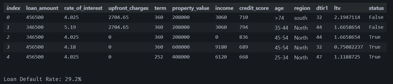
Synthetic data with predicted status column and default rate (~30%).
If the rates are reasonably close, it validates that our synthetic data generation process not only preserves the feature distributions but also maintains the relationships between features that the model learned during training. This comparison is essential for confirming that the synthetic data is suitable for use in simulations, testing, and other applications.
Conclusion
Cumulative Distribution Functions offer a statistically principled and computationally efficient method for generating synthetic data that preserves empirical distributions. By learning the CDFs from real data and using inverse transformation sampling, we can generate unlimited synthetic observations that maintain the statistical properties of the original dataset.
In the game scenario mentioned earlier, generating realistic synthetic loan data enables creating engaging gameplay where players can experience varied scenarios reflecting real-world loan patterns. Players encounter diverse character profiles and loan situations naturally distributed according to historical data, creating authentic challenges and strategic depth.
The technique also extends to other domains like:
- generating synthetic patient data for medical training simulations
- creating diverse game enemy configurations based on real player behavior
- populating test environments with realistic user profiles.
The beauty of this method lies in its balance between statistical foundation and practical simplicity. We preserve empirical distributions without the computational overhead or complexity of more sophisticated generative models, making it ideal for applications where both authenticity and performance matter.
References
This post was written with AI assistance.
You can read this post in Medium.
Similar Posts
-
Loan Default Prediction with Binary Classifier
November 15, 2025 15 minutes read
This post discusses on training a binary classifier with ML.NET using a dataset about defaulted loans from Kaggle. I intend to provide a hands-on introduction to ML.NET for programmers already familiar with the .NET ecosystem, like myself.
-
Eye State Detection in ML.NET - Part 1/2
June 22, 2025 10 minutes read
This two-part blog series explores usage of ONNX models in the ML.NET framework to build a pipeline for detecting eye states (open/closed) in images and video frames captured via webcams. Part one (this post) focuses on leveraging the YuNet Face Detection model to identify and crop the most prominent face.
-
Eye State Detection in ML.NET - Part 2/2
June 22, 2025 10 minutes read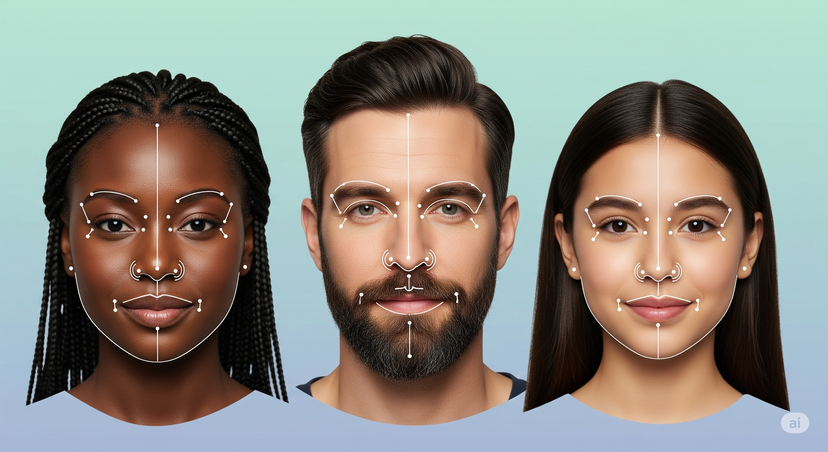
This two-part blog series explores usage of ONNX models in the ML.NET framework to build a pipeline for detecting eye states (open/closed) in images and video frames captured via webcams. Part two (this blog) focuses on utilizing the MediaPipe Face Landmarks Detection model to identify landmarks of left and right eyes in the cropped image, and compute Eye Aspect Ratio (EAR) to detect eye state.